結構化的資料處理

2019-05-11

大綱

讀取CSV
dplyr 的Verbs簡介
資料整合

讀取CSV

CSV的格式

CSV: Comma-Separated Values

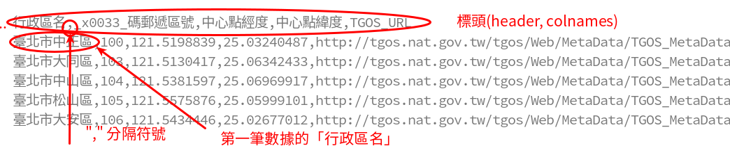
`read.csv`

read.csv("http://homepage.ntu.edu.tw/~wush978/rdataengineer/district_location.csv", 
         header = TRUE, nrows = 6)

##       行政區名 X_x0033_碼郵遞區號 中心點經度 中心點緯度
## 1 臺北市中正區                100   121.5199   25.03240
## 2 臺北市大同區                103   121.5130   25.06342
## 3 臺北市中山區                104   121.5382   25.06970
## 4 臺北市松山區                105   121.5576   25.05999
## 5 臺北市大安區                106   121.5434   25.02677
## 6 臺北市萬華區                108   121.4980   25.02859
##                                                                                                                       TGOS_URL
## 1 http://tgos.nat.gov.tw/tgos/Web/MetaData/TGOS_MetaData_View.aspx?MID=9C715A5CD330360D355AE105F908B29E&SHOW_BACK_BUTTON=false
## 2 http://tgos.nat.gov.tw/tgos/Web/MetaData/TGOS_MetaData_View.aspx?MID=9C715A5CD330360D355AE105F908B29E&SHOW_BACK_BUTTON=false
## 3 http://tgos.nat.gov.tw/tgos/Web/MetaData/TGOS_MetaData_View.aspx?MID=9C715A5CD330360D355AE105F908B29E&SHOW_BACK_BUTTON=false
## 4 http://tgos.nat.gov.tw/tgos/Web/MetaData/TGOS_MetaData_View.aspx?MID=9C715A5CD330360D355AE105F908B29E&SHOW_BACK_BUTTON=false
## 5 http://tgos.nat.gov.tw/tgos/Web/MetaData/TGOS_MetaData_View.aspx?MID=9C715A5CD330360D355AE105F908B29E&SHOW_BACK_BUTTON=false
## 6 http://tgos.nat.gov.tw/tgos/Web/MetaData/TGOS_MetaData_View.aspx?MID=9C715A5CD330360D355AE105F908B29E&SHOW_BACK_BUTTON=false

`read.table`

read.csv("http://homepage.ntu.edu.tw/~wush978/rdataengineer/district_location.csv", 
         sep = ",", header = TRUE, nrows = 6)

##       行政區名 X_x0033_碼郵遞區號 中心點經度 中心點緯度
## 1 臺北市中正區                100   121.5199   25.03240
## 2 臺北市大同區                103   121.5130   25.06342
## 3 臺北市中山區                104   121.5382   25.06970
## 4 臺北市松山區                105   121.5576   25.05999
## 5 臺北市大安區                106   121.5434   25.02677
## 6 臺北市萬華區                108   121.4980   25.02859
##                                                                                                                       TGOS_URL
## 1 http://tgos.nat.gov.tw/tgos/Web/MetaData/TGOS_MetaData_View.aspx?MID=9C715A5CD330360D355AE105F908B29E&SHOW_BACK_BUTTON=false
## 2 http://tgos.nat.gov.tw/tgos/Web/MetaData/TGOS_MetaData_View.aspx?MID=9C715A5CD330360D355AE105F908B29E&SHOW_BACK_BUTTON=false
## 3 http://tgos.nat.gov.tw/tgos/Web/MetaData/TGOS_MetaData_View.aspx?MID=9C715A5CD330360D355AE105F908B29E&SHOW_BACK_BUTTON=false
## 4 http://tgos.nat.gov.tw/tgos/Web/MetaData/TGOS_MetaData_View.aspx?MID=9C715A5CD330360D355AE105F908B29E&SHOW_BACK_BUTTON=false
## 5 http://tgos.nat.gov.tw/tgos/Web/MetaData/TGOS_MetaData_View.aspx?MID=9C715A5CD330360D355AE105F908B29E&SHOW_BACK_BUTTON=false
## 6 http://tgos.nat.gov.tw/tgos/Web/MetaData/TGOS_MetaData_View.aspx?MID=9C715A5CD330360D355AE105F908B29E&SHOW_BACK_BUTTON=false

`read.csv`與`read.table`的注意事項

預設會把character vector轉成factor型態
- 可以用參數stringsAsFactors控制
實務上，R會猜欄位的型態（是character, numeric還是呢？），這很慢
- 可以用參數colClasses直接告訴R答案，讀大資料會快很多

讀取`CSV`的可能錯誤：編碼問題

read.csv(url("http://homepage.ntu.edu.tw/~wush978/rdataengineer/district_location.csv", encoding = "BIG5"), 
         sep = ",", header = TRUE, nrows = 6)

## Warning in read.table(file = file, header = header, sep = sep, quote =
## quote, : 輸入連結 'http://homepage.ntu.edu.tw/~wush978/rdataengineer/
## district_location.csv' 中的輸入不正確

## Warning in read.table(file = file, header = header, sep = sep, quote
## = quote, : incomplete final line found by readTableHeader on 'http://
## homepage.ntu.edu.tw/~wush978/rdataengineer/district_location.csv'

## [1] 銵
## <0 rows> (or 0-length row.names)

解法：先用readLines處理或是用readBin處理後再讀取

讀取`CSV`的可能錯誤：欄位數量不一致

內文包含","或分隔符號
資料有錯

read.csv("http://homepage.ntu.edu.tw/~wush978/rdataengineer/csv-error.csv")

##                        NAME        ID
## Wush Chi-Hsuan Wu d12345678          
## Hsieh               Johnson d12345679

用readLines後手動用strsplit處理

小挑戰

x <- readLines("http://homepage.ntu.edu.tw/~wush978/rdataengineer/csv-error.csv")

請用程式找出兩位的學號

讀取CSV檔案的小撇步: colClasses 參數

read.csv與read.table
colClasses參數可以加速

# source: https://support.spatialkey.com/spatialkey-sample-csv-data/
path <- tempfile(fileext = ".csv.gz")
download.file("http://homepage.ntu.edu.tw/~wush978/rdataengineer/FL_insurance_sample.csv.gz", destfile = path)

讀取CSV檔案的小撇步: colClasses 參數

readLines(gzfile(path), n = 6)

## [1] "policyID,statecode,county,eq_site_limit,hu_site_limit,fl_site_limit,fr_site_limit,tiv_2011,tiv_2012,eq_site_deductible,hu_site_deductible,fl_site_deductible,fr_site_deductible,point_latitude,point_longitude,line,construction,point_granularity"
## [2] "119736,FL,CLAY COUNTY,498960,498960,498960,498960,498960,792148.9,0,9979.2,0,0,30.102261,-81.711777,Residential,Masonry,1"                                                                                                                         
## [3] "448094,FL,CLAY COUNTY,1322376.3,1322376.3,1322376.3,1322376.3,1322376.3,1438163.57,0,0,0,0,30.063936,-81.707664,Residential,Masonry,3"                                                                                                             
## [4] "206893,FL,CLAY COUNTY,190724.4,190724.4,190724.4,190724.4,190724.4,192476.78,0,0,0,0,30.089579,-81.700455,Residential,Wood,1"                                                                                                                      
## [5] "333743,FL,CLAY COUNTY,0,79520.76,0,0,79520.76,86854.48,0,0,0,0,30.063236,-81.707703,Residential,Wood,3"                                                                                                                                            
## [6] "172534,FL,CLAY COUNTY,0,254281.5,0,254281.5,254281.5,246144.49,0,0,0,0,30.060614,-81.702675,Residential,Wood,1"

system.time(
  FL <- read.csv(gzfile(path), header = TRUE)
)

##    user  system elapsed 
##   0.288   0.010   0.298

讀取CSV檔案的小撇步: colClasses 參數

system.time({
  FL.head <- read.csv(gzfile("FL_insurance_sample.csv.gz"), header = TRUE, nrows = 6)
  .col <- sapply(FL.head, class)
  .col[.col == "integer"] <- "numeric"
  FL <- read.csv(gzfile("FL_insurance_sample.csv.gz"), header = TRUE, colClasses = .col)
})

##    user  system elapsed 
##   0.170   0.008   0.184

讀取CSV檔案的小撇步: colClasses 參數

head(FL)

##   policyID statecode      county eq_site_limit hu_site_limit fl_site_limit
## 1   119736        FL CLAY COUNTY      498960.0     498960.00      498960.0
## 2   448094        FL CLAY COUNTY     1322376.3    1322376.30     1322376.3
## 3   206893        FL CLAY COUNTY      190724.4     190724.40      190724.4
## 4   333743        FL CLAY COUNTY           0.0      79520.76           0.0
## 5   172534        FL CLAY COUNTY           0.0     254281.50           0.0
## 6   785275        FL CLAY COUNTY           0.0     515035.62           0.0
##   fr_site_limit   tiv_2011   tiv_2012 eq_site_deductible
## 1      498960.0  498960.00  792148.90                  0
## 2     1322376.3 1322376.30 1438163.57                  0
## 3      190724.4  190724.40  192476.78                  0
## 4           0.0   79520.76   86854.48                  0
## 5      254281.5  254281.50  246144.49                  0
## 6           0.0  515035.62  884419.17                  0
##   hu_site_deductible fl_site_deductible fr_site_deductible point_latitude
## 1             9979.2                  0                  0       30.10226
## 2                0.0                  0                  0       30.06394
## 3                0.0                  0                  0       30.08958
## 4                0.0                  0                  0       30.06324
## 5                0.0                  0                  0       30.06061
## 6                0.0                  0                  0       30.06324
##   point_longitude        line construction point_granularity
## 1       -81.71178 Residential      Masonry                 1
## 2       -81.70766 Residential      Masonry                 3
## 3       -81.70046 Residential         Wood                 1
## 4       -81.70770 Residential         Wood                 3
## 5       -81.70267 Residential         Wood                 1
## 6       -81.70770 Residential      Masonry                 3

Database

作業在 Windows 上的 3.5 系列有bug，修復中
- 請Windows使用者用別的版本的R跑作業
什麼時候用 Database?
- 記憶體不夠
- 需要Transaction(多個操作中，只要一個失敗就全部復原)

Transaction

線上的資料處理上，在「容錯」上非常重要的「特性」
範例：
- 假設每小時產生一個檔案

out.path <- sprintf("%s.csv", format(Sys.time(), "%Y-%m-%d-%H"))
# do something
write(data, file = out.path)

Transaction

線上的資料處理上，在「容錯」上非常重要的「特性」
範例：
- 假設每小時產生一個檔案
- 寫入到一半的時候發生錯誤（斷電、當機）
- 自動重開機後又繼續跑，產生新的檔案
- 哪些檔案是錯的？

Transaction

out.path <- format(Sys.time(), "%Y-%m-%d-%H.csv")
out.path.tmp <- paste(out.path, "tmp", sep = ".")
write(data, file = out.path.tmp)
# rename is transaction
file.rename(out.path.tmp, out.path)

XML Tables

XML::readHTMLTable
XML 是比較老牌的XML處理工具
- 資料結構比xml2更難懂，但是比較穩(?)
- 如果資料來源是結構化的HTML表格，XML::readHTMLTable很方便

2018 縣市長大選台北即時估票

外差估票程式
1. 從中選會的網頁上抓候選人的得票數
2. 利用各正區現有的得票率當機準，依照「已開票」與「未開票」的比率放大
3. 推估最終候選人的得票
4. 可惜現在網頁格式不一致，所以會跑出NA XD
紀錄

data.frame

由list物件擴充而成
- list + attributes
在R 語言中，處理「表格」(table)資料
- 表格 v.s. 矩陣、陣列
視覺化：ggplot2
許多進階分析的入口
- 例：迴歸分析(lm)
- 將表格的變數轉換成數學上的矩陣：model.matrix $\hat{\beta} = (X^TX)^{-1}(X^Ty)$

data.frame 的 Create

注意參數： stringsAsFactors

data.frame(student.id = 1:5, math.score = rpois(5, 5))

##   student.id math.score
## 1          1          3
## 2          2          8
## 3          3          3
## 4          4          4
## 5          5          5

data.frame 的 Create

df <- read.csv(
  url("https://raw.githubusercontent.com/wush978/DataScienceAndR/course/01-RBasic-07-Loading-Dataset/A_LVR_LAND_A.CSV", encoding = "BIG5"), 
  nrows = 6, header = TRUE)
df[,1:3]

##   鄉鎮市區        交易標的                土地區段位置或建物區門牌
## 1   文山區 房地(土地+建物) 臺北市文山區木柵路二段109巷100弄61~90號
## 2   中正區 房地(土地+建物)                臺北市中正區南海路1~30號
## 3   中正區 房地(土地+建物)       臺北市中正區重慶南路三段121~150號
## 4   文山區 房地(土地+建物)        臺北市文山區指南路三段32巷1~30號
## 5   文山區 房地(土地+建物)   臺北市文山區羅斯福路五段92巷1弄1~30號
## 6   文山區 房地(土地+建物)            臺北市文山區秀明路二段1~30號

data.frame 的 Read

list的Read: [、[[與$

df["鄉鎮市區"]

##   鄉鎮市區
## 1   文山區
## 2   中正區
## 3   中正區
## 4   文山區
## 5   文山區
## 6   文山區

data.frame 的 Read

list的Read: [、[[與$

df[["鄉鎮市區"]]

## [1] 文山區 中正區 中正區 文山區 文山區 文山區
## Levels: 文山區 中正區

data.frame 的 Read

list的Read: [、[[與$

df$`鄉鎮市區`

## [1] 文山區 中正區 中正區 文山區 文山區 文山區
## Levels: 文山區 中正區

data.frame 的 Read

[: 仍然是data.frame
[[、$: data.frame(list)會被打破

data.frame 的 Read

matrix的Read: [

df[1,1]

## [1] 文山區
## Levels: 文山區 中正區

df[1:2,1]

## [1] 文山區 中正區
## Levels: 文山區 中正區

df[1,1:2]

##   鄉鎮市區        交易標的
## 1   文山區 房地(土地+建物)

data.frame 的 Read

matrix的Read: [
- 應仍然是data.frame
- 參數drop = TRUE(預設)當欄位方向的維度為1時，會自動把data.frame轉成向量

df[1:2,1:2]

##   鄉鎮市區        交易標的
## 1   文山區 房地(土地+建物)
## 2   中正區 房地(土地+建物)

df[1,1,drop = FALSE]

##   鄉鎮市區
## 1   文山區

data.frame 的 Read

drop = TRUE 是好事嘛？
- Hadley 主導的 tidyverse
- 不是所有人都喜歡… tibbles are not data.frames

data.frame 的 Update

Read + <-

df <- data.frame(
  id = 1:5, 
  score = sample(1:10, 5, TRUE))
df

##   id score
## 1  1     4
## 2  2     8
## 3  3     5
## 4  4     8
## 5  5     5

df$score <- scale(df$score)
df

##   id      score
## 1  1 -1.0690450
## 2  2  1.0690450
## 3  3 -0.5345225
## 4  4  1.0690450
## 5  5 -0.5345225

data.frame 的 Delete

反向Read
Read + <- NULL

df[-1,] # df[2:5,]

##   id      score
## 2  2  1.0690450
## 3  3 -0.5345225
## 4  4  1.0690450
## 5  5 -0.5345225

df$score <- NULL
df

##   id
## 1  1
## 2  2
## 3  3
## 4  4
## 5  5

範例

iris的資料中
- Sepal.Length的平均
- 各種Species的平均Sepal.Length
- 建立新的欄位：std.Sepal.Length是標準化後的Sepal.Length
- 建立新的欄位：std.Sepal.Length是依照個別Species作標準化後的Sepal.Length

範例

各種Species的平均Sepal.Length

ans <- c()
for(.sp in levels(iris$Species)) {
  .i <- iris$Species == .sp
  ans[.sp] <- mean(iris$Sepal.Length[.i])
}
ans

##     setosa versicolor  virginica 
##      5.006      5.936      6.588

範例

各種Species的平均Sepal.Length

# you can use `lapply` and then `unlist`
sapply(levels(iris$Species), function(.sp) {
  .i <- iris$Species == .sp
  mean(iris$Sepal.Length[.i])
})

##     setosa versicolor  virginica 
##      5.006      5.936      6.588

範例

各種Species的平均Sepal.Length

. <- split(iris, iris$Species)
. <- lapply(., "[[", "Sepal.Length")
sapply(., mean)

##     setosa versicolor  virginica 
##      5.006      5.936      6.588

範例

各種Species的平均Sepal.Length

aggregate(Sepal.Length ~ Species, iris, mean)

##      Species Sepal.Length
## 1     setosa        5.006
## 2 versicolor        5.936
## 3  virginica        6.588

要理解這段expression，同學需要學會：
- formula object
- Aggregation functions

範例

建立新的欄位：std.Sepal.Length是標準化後的Sepal.Length

ans <- iris # to backup the original object, we modify after copying
. <- iris$Sepal.Length - mean(iris$Sepal.Length)
. <- . / sd(iris$Sepal.Length)
ans$std.Sepal.Length <- .
ans[c(1,2,51,52,101,102),6,drop=FALSE]

##     std.Sepal.Length
## 1        -0.89767388
## 2        -1.13920048
## 51        1.39682886
## 52        0.67224905
## 101       0.55148575
## 102      -0.05233076

範例

建立新的欄位：std.Sepal.Length是標準化後的Sepal.Length

ans <- iris # to backup the original object, we modify after copying
ans$std.Sepal.Length <- scale(iris$Sepal.Length)
ans[c(1,2,51,52,101,102),6,drop=FALSE]

##     std.Sepal.Length
## 1        -0.89767388
## 2        -1.13920048
## 51        1.39682886
## 52        0.67224905
## 101       0.55148575
## 102      -0.05233076

範例

建立新的欄位：std.Sepal.Length是依照個別Species作標準化後的Sepal.Length

. <- iris$Sepal.Length
for(.sp in levels(iris$Species)) {
  .i <- iris$Species == .sp
  .[.i] <- scale(.[.i])
}
ans <- iris
ans$std.Sepal.Length <- .
ans[c(1,2,51,52,101,102),6,drop=FALSE]

##     std.Sepal.Length
## 1          0.2666745
## 2         -0.3007180
## 51         2.0613318
## 52         0.8989266
## 101       -0.4529159
## 102       -1.2392283

範例

建立新的欄位：std.Sepal.Length是依照個別Species作標準化後的Sepal.Length

# This code will not work if the species is not ordered
. <- lapply(levels(iris$Species), function(.sp) {
  .i <- iris$Species == .sp
  scale(iris$Sepal.Length[.i])
})
ans <- iris
ans$std.Sepal.Length <- unlist(.)
ans[c(1,2,51,52,101,102),6,drop=FALSE]

##     std.Sepal.Length
## 1          0.2666745
## 2         -0.3007180
## 51         2.0613318
## 52         0.8989266
## 101       -0.4529159
## 102       -1.2392283

dplyr

參考SQL 資料庫系統對結構化資料的操作做設計

一般企業儲存結構化資料的工具
- 儲存所有資料的工具
- Transaction: 操作要嘛成功，要嘛無效
SQL 資料庫的結構與操作是有數學代數在背後(Relational Algebra)
R的data.frame v.s. SQL 資料庫
- memory v.s. disk
- indexing
- column based v.s. row based
一致的設計，讓同學可以透過dplyr的語法寫SQL
- 老師的經驗：比起用dplyr操作Database，還是直接寫 SQL 比較簡單… 但是可順便學SQL
- 有SQL經驗的同學可以快速上手R 的data.frame

dplyr 沒有完全相容於 data.frame

有時候，輸出的table不再是data.frame
- 為了效能
- 為了設計
- 因為Hadley(?)
有必要時可以使用as.data.frame

Single Table verbs

Read / Delete
- filter、slice
- select
- sample_n、sample_frac
Update
- mutate
- arrange
Others
- summarise
- group_by
- do

針對列作篩選：filter

head(iris[iris$Sepal.Length > 3,1,drop=FALSE])

##   Sepal.Length
## 1          5.1
## 2          4.9
## 3          4.7
## 4          4.6
## 5          5.0
## 6          5.4

head(filter(iris, Sepal.Length > 3)[,1,drop=FALSE])

##   Sepal.Length
## 1          5.1
## 2          4.9
## 3          4.7
## 4          4.6
## 5          5.0
## 6          5.4

針對列作篩選：filter

在dplyr的函數中，iris$可以被省略
- 解析順序：欄位名稱 –> 變數名稱
filter的第一個參數是要處理的data.frame物件
- 所有的dplyr函數都是這樣設計
filter的其他參數必須是一個布林向量，並且長度一致
- 所有的這類參數，都是TRUE的位置，才會回傳

針對列作篩選：filter

head(filter(iris, Sepal.Length > 3, Sepal.Width < 3.5))

##   Sepal.Length Sepal.Width Petal.Length Petal.Width Species
## 1          4.9         3.0          1.4         0.2  setosa
## 2          4.7         3.2          1.3         0.2  setosa
## 3          4.6         3.1          1.5         0.2  setosa
## 4          4.6         3.4          1.4         0.3  setosa
## 5          5.0         3.4          1.5         0.2  setosa
## 6          4.4         2.9          1.4         0.2  setosa

針對列作篩選：filter

head(filter(iris, Sepal.Length > 3, Sepal.Width < 3.5, Species == "versicolor"))

##   Sepal.Length Sepal.Width Petal.Length Petal.Width    Species
## 1          7.0         3.2          4.7         1.4 versicolor
## 2          6.4         3.2          4.5         1.5 versicolor
## 3          6.9         3.1          4.9         1.5 versicolor
## 4          5.5         2.3          4.0         1.3 versicolor
## 5          6.5         2.8          4.6         1.5 versicolor
## 6          5.7         2.8          4.5         1.3 versicolor

針對列作篩選：filter

a <- iris$Sepal.Length + iris$Sepal.Width
head(filter(iris, Sepal.Length > 3, Sepal.Width < 3.5, a < 8))

##   Sepal.Length Sepal.Width Petal.Length Petal.Width Species
## 1          4.9         3.0          1.4         0.2  setosa
## 2          4.7         3.2          1.3         0.2  setosa
## 3          4.6         3.1          1.5         0.2  setosa
## 4          4.4         2.9          1.4         0.2  setosa
## 5          4.8         3.0          1.4         0.1  setosa
## 6          4.3         3.0          1.1         0.1  setosa

針對列作篩選：slice

slice(iris, 1:6)

##   Sepal.Length Sepal.Width Petal.Length Petal.Width Species
## 1          5.1         3.5          1.4         0.2  setosa
## 2          4.9         3.0          1.4         0.2  setosa
## 3          4.7         3.2          1.3         0.2  setosa
## 4          4.6         3.1          1.5         0.2  setosa
## 5          5.0         3.6          1.4         0.2  setosa
## 6          5.4         3.9          1.7         0.4  setosa

針對列作抽樣：`sample_n`、`sample_frac`

sample_n(iris, 6)[,1,drop=FALSE]

##   Sepal.Length
## 1          5.6
## 2          6.5
## 3          4.4
## 4          5.7
## 5          6.1
## 6          6.0

sample_frac(iris, 0.04)[,1,drop=FALSE]

##   Sepal.Length
## 1          7.6
## 2          6.3
## 3          6.0
## 4          6.3
## 5          6.0
## 6          6.6

針對欄位作篩選：select

head(select(iris, Sepal.Length))

##   Sepal.Length
## 1          5.1
## 2          4.9
## 3          4.7
## 4          4.6
## 5          5.0
## 6          5.4

針對欄位作篩選：select

head(select(iris, Sepal.Length, Sepal.Width))

##   Sepal.Length Sepal.Width
## 1          5.1         3.5
## 2          4.9         3.0
## 3          4.7         3.2
## 4          4.6         3.1
## 5          5.0         3.6
## 6          5.4         3.9

針對欄位作篩選：select

head(select(iris, starts_with("Sepal")))

##   Sepal.Length Sepal.Width
## 1          5.1         3.5
## 2          4.9         3.0
## 3          4.7         3.2
## 4          4.6         3.1
## 5          5.0         3.6
## 6          5.4         3.9

針對欄位作篩選：select

head(select(iris, Sepal.Length:Petal.Length))

##   Sepal.Length Sepal.Width Petal.Length
## 1          5.1         3.5          1.4
## 2          4.9         3.0          1.4
## 3          4.7         3.2          1.3
## 4          4.6         3.1          1.5
## 5          5.0         3.6          1.4
## 6          5.4         3.9          1.7

針對欄位作篩選：select

反向操作

head(select(iris, -Sepal.Length))

##   Sepal.Width Petal.Length Petal.Width Species
## 1         3.5          1.4         0.2  setosa
## 2         3.0          1.4         0.2  setosa
## 3         3.2          1.3         0.2  setosa
## 4         3.1          1.5         0.2  setosa
## 5         3.6          1.4         0.2  setosa
## 6         3.9          1.7         0.4  setosa

針對欄位作篩選：select

rename

head(select(iris, SL = Sepal.Length))

##    SL
## 1 5.1
## 2 4.9
## 3 4.7
## 4 4.6
## 5 5.0
## 6 5.4

更改資料(向量化)

mutate

head(mutate(iris, Sepal = mean(Sepal.Length + Sepal.Width)))

##   Sepal.Length Sepal.Width Petal.Length Petal.Width Species    Sepal
## 1          5.1         3.5          1.4         0.2  setosa 8.900667
## 2          4.9         3.0          1.4         0.2  setosa 8.900667
## 3          4.7         3.2          1.3         0.2  setosa 8.900667
## 4          4.6         3.1          1.5         0.2  setosa 8.900667
## 5          5.0         3.6          1.4         0.2  setosa 8.900667
## 6          5.4         3.9          1.7         0.4  setosa 8.900667

更改資料(向量化)

mutate

head(mutate(iris, Sepal.Length = as.character(Sepal.Length)))

##   Sepal.Length Sepal.Width Petal.Length Petal.Width Species
## 1          5.1         3.5          1.4         0.2  setosa
## 2          4.9         3.0          1.4         0.2  setosa
## 3          4.7         3.2          1.3         0.2  setosa
## 4          4.6         3.1          1.5         0.2  setosa
## 5            5         3.6          1.4         0.2  setosa
## 6          5.4         3.9          1.7         0.4  setosa

Aggregation: summarise

150 rows –> 1 row

summarise(iris, mean(Sepal.Length))

##   mean(Sepal.Length)
## 1           5.843333

Aggregation: summarise

150 rows –> 2 row? error

summarise(iris, range(Sepal.Length))

## Error: Column `range(Sepal.Length)` must be length 1 (a summary value), not 2

Aggregation: do

150 rows –> 2 row
. is iris here

do(iris, data.frame(rSL = range(.$Sepal.Length)))

##   rSL
## 1 4.3
## 2 7.9

Aggregation的目的

why summarise?

summarise(iris, mean(Sepal.Length))[[1]]

## [1] 5.843333

mean(iris$Sepal.Length)

## [1] 5.843333

Because summarise/do recognize group_by

Aggregation: `group_by`

Default group is iris
- mutate/summarise/do apply the expressions to the group
We can split iris to several groups based on specific (categorical) variable
- character or factor

group_by(iris, Species) # Nothing happens

## # A tibble: 150 x 5
## # Groups:   Species [3]
##    Sepal.Length Sepal.Width Petal.Length Petal.Width Species
##           <dbl>       <dbl>        <dbl>       <dbl> <fct>  
##  1          5.1         3.5          1.4         0.2 setosa 
##  2          4.9         3            1.4         0.2 setosa 
##  3          4.7         3.2          1.3         0.2 setosa 
##  4          4.6         3.1          1.5         0.2 setosa 
##  5          5           3.6          1.4         0.2 setosa 
##  6          5.4         3.9          1.7         0.4 setosa 
##  7          4.6         3.4          1.4         0.3 setosa 
##  8          5           3.4          1.5         0.2 setosa 
##  9          4.4         2.9          1.4         0.2 setosa 
## 10          4.9         3.1          1.5         0.1 setosa 
## # … with 140 more rows

Aggregation: `group_by` + `summarise`

. <- group_by(iris, Species)
summarise(., mean(Sepal.Length))

## # A tibble: 3 x 2
##   Species    `mean(Sepal.Length)`
##   <fct>                     <dbl>
## 1 setosa                     5.01
## 2 versicolor                 5.94
## 3 virginica                  6.59

`filter` –> `group_by`

.x1 <- filter(iris, Species == "setosa")
summarise(.x1, mean(Sepal.Length))

##   mean(Sepal.Length)
## 1              5.006

`filter` –> `group_by`

.x1 <- filter(iris, Species == "setosa")
.x2 <- filter(iris, Species == "versicolor")
.x3 <- filter(iris, Species == "virginica")
rbind(
  summarise(.x1, mean(Sepal.Length)),
  summarise(.x2, mean(Sepal.Length)),
  summarise(.x3, mean(Sepal.Length))
)

##   mean(Sepal.Length)
## 1              5.006
## 2              5.936
## 3              6.588

Aggregation

透過group_by把原本的data.frame切割成若干個groups
之後的verbs會各自對個別的groups運作，一個group跑一次(會有多個data.frame)，最後再rbind成為單一的data.frame

Aggregation: `group_by` + `summarise`

. <- group_by(iris, Species)
summarise(., mean(Sepal.Length), mean(Sepal.Width))

## # A tibble: 3 x 3
##   Species    `mean(Sepal.Length)` `mean(Sepal.Width)`
##   <fct>                     <dbl>               <dbl>
## 1 setosa                     5.01                3.43
## 2 versicolor                 5.94                2.77
## 3 virginica                  6.59                2.97

Aggregation: `group_by` + `summarise`

結果的維度： group 的數量 $\times$ ?
- ?是所有在資料中出現的組合的個數

. <- group_by(iris, Species, floor(Petal.Length))
summarise(., mean(Sepal.Length), mean(Sepal.Width))

## # A tibble: 7 x 4
## # Groups:   Species [3]
##   Species    `floor(Petal.Length)` `mean(Sepal.Length)` `mean(Sepal.Width)`
##   <fct>                      <dbl>                <dbl>               <dbl>
## 1 setosa                         1                 5.01                3.43
## 2 versicolor                     3                 5.35                2.49
## 3 versicolor                     4                 6.09                2.85
## 4 versicolor                     5                 6.35                2.85
## 5 virginica                      4                 5.85                2.8 
## 6 virginica                      5                 6.44                2.94
## 7 virginica                      6                 7.43                3.16

Aggregation: `group_by` + `do`

. <- group_by(iris, Species)
do(., data.frame(type = c("min", "max"), r1 = range(.$Sepal.Length), r2 = range(.$Sepal.Width)))

## # A tibble: 6 x 4
## # Groups:   Species [3]
##   Species    type     r1    r2
##   <fct>      <fct> <dbl> <dbl>
## 1 setosa     min     4.3   2.3
## 2 setosa     max     5.8   4.4
## 3 versicolor min     4.9   2  
## 4 versicolor max     7     3.4
## 5 virginica  min     4.9   2.2
## 6 virginica  max     7.9   3.8

Aggregation: `group_by` + `summarise`

利用browser詳細了解group_by與summarise

. <- group_by(iris, Species)
summarise(., SL = {
  browser()
  mean(Sepal.Length)
})

Aggregation: `group_by` + `do`

利用browser詳細了解group_by與do
在中斷點(Browser[1]>之下)可檢閱變數.

. <- group_by(iris, Species)
do(., {
  browser()
  data.frame(r1 = range(Sepal.Length))
})

小挑戰

請嘗試用dplyr的函數，從iris的資料中計算：
- Sepal.Length的平均(mean)
- 各種Species的平均Sepal.Length(mean)
- 建立新的欄位：std.Sepal.Length是標準化後的Sepal.Length(scale)
- 建立新的欄位：std.Sepal.Length是依照個別Species作標準化後的Sepal.Length(scale)

參考答案

建立新的欄位：std.Sepal.Length是標準化後的Sepal.Length

mutate(iris, std.Sepal.Length = scale(Sepal.Length))[c(1,2,51,52,101,102),4:6]

##     Petal.Width    Species std.Sepal.Length
## 1           0.2     setosa      -0.89767388
## 2           0.2     setosa      -1.13920048
## 51          1.4 versicolor       1.39682886
## 52          1.5 versicolor       0.67224905
## 101         2.5  virginica       0.55148575
## 102         1.9  virginica      -0.05233076

參考答案

建立新的欄位：std.Sepal.Length是依照個別Species作標準化後的Sepal.Length

. <- group_by(iris, Species)
mutate(., std.Sepal.Length = scale(Sepal.Length))[c(1,2,51,52,101,102),4:6]

## # A tibble: 6 x 3
## # Groups:   Species [3]
##   Petal.Width Species    std.Sepal.Length
##         <dbl> <fct>                 <dbl>
## 1         0.2 setosa                0.267
## 2         0.2 setosa               -0.301
## 3         1.4 versicolor            2.06 
## 4         1.5 versicolor            0.899
## 5         2.5 virginica            -0.453
## 6         1.9 virginica            -1.24

從`dplyr`到SQL

每一個Single Table Verbs會對到SQL Keyword, Ex:
- select –> SELECT
- filter –> WHERE

從`dplyr`到SQL

suppressPackageStartupMessages(
  library(sqldf)
  )
sqldf("
SELECT `Sepal.Length` FROM iris 
WHERE Species = 'setosa' LIMIT 6"
)

##   Sepal.Length
## 1          5.1
## 2          4.9
## 3          4.7
## 4          4.6
## 5          5.0
## 6          5.4

. <- filter(iris, Species == "setosa")
. <- select(., Sepal.Length)
slice(., 1:6)

##   Sepal.Length
## 1          5.1
## 2          4.9
## 3          4.7
## 4          4.6
## 5          5.0
## 6          5.4

從`dplyr`到SQL

同學仍然需要找機會學習SQL的expression規則
- SQL 在資料科學是比 R 還重要的存在
- 懂 dplyr 後學 SQL 的概念會很快，因為背後的設計相同（把那些verbs換個名詞而已）
SQL 和 GROUP BY 與 dplyr 的 group_by都是 aggregation functions
- 但是在R 中我們可以用中斷點作探索，更快的理解aggregation functions

從`dplyr`到SQL

suppressPackageStartupMessages(library(dbplyr))
library(RSQLite)
src <- src_sqlite(tempfile(fileext = ".db"), create = TRUE)
copy_to(src, iris)
iris.db <- tbl(src, "iris")
filter(iris.db, Species == "versicolor")

## # Source:   lazy query [?? x 5]
## # Database: sqlite 3.22.0
## #   [/var/folders/x6/z8_v_l4x1qjdwmzkc98sj0lw0000gp/T//Rtmp45nxGb/file1858c189d9a62.db]
##    Sepal.Length Sepal.Width Petal.Length Petal.Width Species   
##           <dbl>       <dbl>        <dbl>       <dbl> <chr>     
##  1          7           3.2          4.7         1.4 versicolor
##  2          6.4         3.2          4.5         1.5 versicolor
##  3          6.9         3.1          4.9         1.5 versicolor
##  4          5.5         2.3          4           1.3 versicolor
##  5          6.5         2.8          4.6         1.5 versicolor
##  6          5.7         2.8          4.5         1.3 versicolor
##  7          6.3         3.3          4.7         1.6 versicolor
##  8          4.9         2.4          3.3         1   versicolor
##  9          6.6         2.9          4.6         1.3 versicolor
## 10          5.2         2.7          3.9         1.4 versicolor
## # … with more rows

從`dplyr`到SQL

aggregation 會受到 database 的限制

suppressPackageStartupMessages(library(dbplyr))
library(RSQLite)
src <- src_sqlite(tempfile(fileext = ".db"), create = TRUE)
copy_to(src, iris)
iris.db <- tbl(src, "iris")
. <- group_by(iris.db, Species)
do(., data.frame(r1 = range(.$Sepal.Length)))

## Error: No more ticks

Table 的種類

Wide Table

row is an instance
columns are attributes

df.wide <- data.frame(
  id = c("Bob", "John", "Anderson"), 
  math = c(80, 85, 90), 
  science = c(75, 60, 100)
  )
df.wide

##         id math science
## 1      Bob   80      75
## 2     John   85      60
## 3 Anderson   90     100

Tall Table

又稱為 narrow 或 stacked data

library(reshape2)
df.tall <- melt(df.wide, variable.name = "subject", value.name = "score")

## Using id as id variables

df.tall

##         id subject score
## 1      Bob    math    80
## 2     John    math    85
## 3 Anderson    math    90
## 4      Bob science    75
## 5     John science    60
## 6 Anderson science   100

Tall Table –> Wide Table (Pivoting)

library(reshape2)
dcast(df.tall, id ~ subject)

## Using score as value column: use value.var to override.

##         id math science
## 1 Anderson   90     100
## 2      Bob   80      75
## 3     John   85      60

# stats::reshape(df.tall, idvar = "id", 
#   v.names = "score", timevar = "subject", 
#   direction = "wide")

wide table 在現實生活很常見，但是會有什麼問題呢？

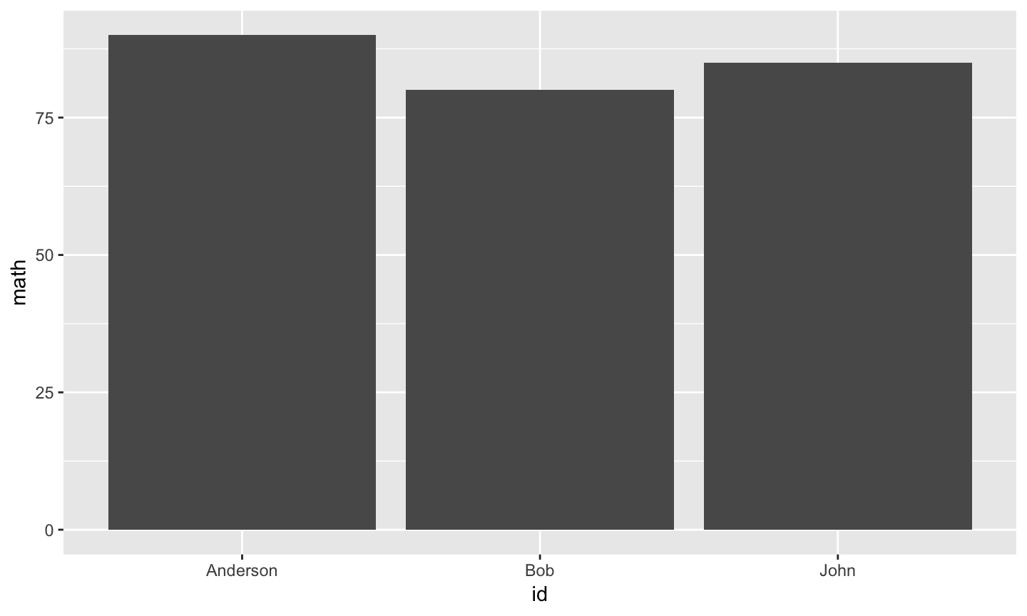
wide table 的限制，以ggplot2為例

在df.wide上比較math 或 science 很容易

library(ggplot2)
ggplot(df.wide, aes(x = id, y = math)) +
  geom_bar(stat = "identity")

wide table 的限制，以ggplot2為例

但是怎麼同時比較 math 與 science?

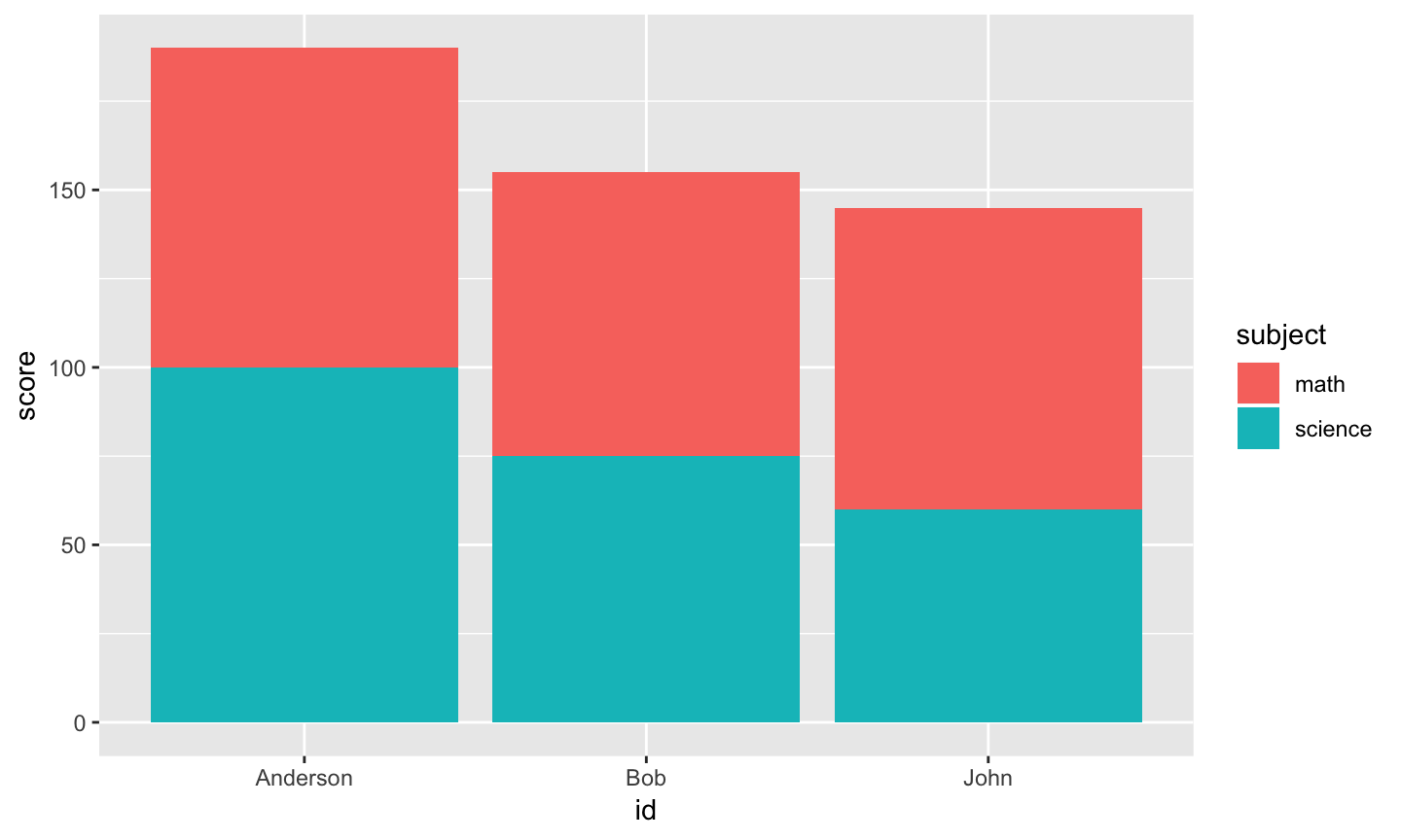
範例：ggplot2

ggplot2 is more friendly to tall table

library(ggplot2)
ggplot(df.tall, aes(x = id, y = score, fill = subject)) +
  geom_bar(stat = "identity")

Wide Table –> Tall Table

library(reshape2)
df.tall <- melt(df.wide, variable.name = "subject", value.name = "score")

Wide Table –> Tall Table

. <- iris
.$id <- rownames(iris)
iris.tall <- melt(
  ., variable.name = "measurement", value.name = "value", 
  id.vars = "id", stringsAsFactors = FALSE)

## Warning: attributes are not identical across measure variables; they will
## be dropped

filter(iris.tall, id == "1")

##   id  measurement  value
## 1  1 Sepal.Length    5.1
## 2  1  Sepal.Width    3.5
## 3  1 Petal.Length    1.4
## 4  1  Petal.Width    0.2
## 5  1      Species setosa

Wide Table v.s. Tall Table

Wide Table 每一列要對應到一個instance
Tall Table 要有一個欄位（會重複）代表identity
- 相同的identity代表相同的instance
我不知道對於這兩種table的嚴謹定義。實務上，也是有Table會介於兩者之間
重點在於了解wide table與tall table適合使用的情境
- 必要時需要作轉型

df.tall

##         id subject score
## 1      Bob    math    80
## 2     John    math    85
## 3 Anderson    math    90
## 4      Bob science    75
## 5     John science    60
## 6 Anderson science   100

小挑戰

請問iris算是 wide table 還是 tall table?

slice(iris, c(1, 2, 51, 52, 101, 102))

##   Sepal.Length Sepal.Width Petal.Length Petal.Width    Species
## 1          5.1         3.5          1.4         0.2     setosa
## 2          4.9         3.0          1.4         0.2     setosa
## 3          7.0         3.2          4.7         1.4 versicolor
## 4          6.4         3.2          4.5         1.5 versicolor
## 5          6.3         3.3          6.0         2.5  virginica
## 6          5.8         2.7          5.1         1.9  virginica

小挑戰

請問cars算是 wide table 還是 tall table?

cars

##    speed dist
## 1      4    2
## 2      4   10
## 3      7    4
## 4      7   22
## 5      8   16
## 6      9   10
## 7     10   18
## 8     10   26
## 9     10   34
## 10    11   17
## 11    11   28
## 12    12   14
## 13    12   20
## 14    12   24
## 15    12   28
## 16    13   26
## 17    13   34
## 18    13   34
## 19    13   46
## 20    14   26
## 21    14   36
## 22    14   60
## 23    14   80
## 24    15   20
## 25    15   26
## 26    15   54
## 27    16   32
## 28    16   40
## 29    17   32
## 30    17   40
## 31    17   50
## 32    18   42
## 33    18   56
## 34    18   76
## 35    18   84
## 36    19   36
## 37    19   46
## 38    19   68
## 39    20   32
## 40    20   48
## 41    20   52
## 42    20   56
## 43    20   64
## 44    22   66
## 45    23   54
## 46    24   70
## 47    24   92
## 48    24   93
## 49    24  120
## 50    25   85

Wide Table v.s. Tall Table

Wide Table的好處
- 比較容易閱讀、空間比較省
- 適合作aggregation
- 適合作modeling
Tall Table的好處
- 增加測量的類型時，不用對舊的資料造成破壞
- ggplot2

對`iris`計算各個Species的平均

. <- group_by(iris, Species)
summarise_all(., mean)

## # A tibble: 3 x 5
##   Species    Sepal.Length Sepal.Width Petal.Length Petal.Width
##   <fct>             <dbl>       <dbl>        <dbl>       <dbl>
## 1 setosa             5.01        3.43         1.46       0.246
## 2 versicolor         5.94        2.77         4.26       1.33 
## 3 virginica          6.59        2.97         5.55       2.03

對`iris.tall`計算各個Species的平均

species <- filter(iris.tall, measurement == "Species")
species <- unique(species$value)
measurements <- unique(iris.tall$measurement)
measurements <- as.character(measurements)
measurements <- setdiff(measurements, "Species")
result <- data.frame(
  Species = species
)
for(m in measurements) {
  result[[m]] <- numeric(nrow(result))
}
for(i in 1:length(species)) {
  current.species <- filter(iris.tall, measurement == "Species", value == species[i])
  #.$id
  for(j in c("Sepal.Length", "Sepal.Width", "Petal.Length", "Petal.Width")) {
    . <- filter(iris.tall, measurement == j, id %in% current.species$id)
    result[[j]][i] <- mean(as.numeric(.$value))
  }
}

對`iris.tall`計算各個Species的平均

. <- stats::reshape(
  iris.tall, v.names = "value", 
  timevar = "measurement", direction = "wide")
. <- select(., value.Sepal.Length : value.Species)
for(j in 1:4) {
  .[[j]] <- as.numeric(.[[j]])
}
. <- group_by(., value.Species)
summarise_all(., mean)

## # A tibble: 3 x 5
##   value.Species value.Sepal.Len… value.Sepal.Wid… value.Petal.Len…
##   <chr>                    <dbl>            <dbl>            <dbl>
## 1 setosa                    5.01             3.43             1.46
## 2 versicolor                5.94             2.77             4.26
## 3 virginica                 6.59             2.97             5.55
## # … with 1 more variable: value.Petal.Width <dbl>

pipeline operator

資料處理就是一個連續組合動作

. <- filter(iris, Species == "setosa")
. <- select(., Sepal.Length)
head(., 6)

##   Sepal.Length
## 1          5.1
## 2          4.9
## 3          4.7
## 4          4.6
## 5          5.0
## 6          5.4

運用中間變數

. 永遠是中間變數，不會混用
- 常見的還有x、y、i…
- 但是中間變數的名字越多，越容易混淆

for(i in ...) {
  ...
  for(i in ...) { # i is duplicated
    ... 
  }
  ... # i has been changed
}

解決辦法：保持environment的乾淨

中間變數一律用.開頭
- 預設會隱藏這些變數
nested function call

head(select(filter(iris, Species == "setosa"), Sepal.Length), 6)

##   Sepal.Length
## 1          5.1
## 2          4.9
## 3          4.7
## 4          4.6
## 5          5.0
## 6          5.4

解決辦法：pipeline operator `%>%`

%>%會把左邊的expression的結果，當成右邊函數呼叫的第一個參數
- 參數對應的方式：先比對名稱，再按照順序

filter(iris, Species == "setosa") %>%
  select(Sepal.Length) %>%
  head(6)

##   Sepal.Length
## 1          5.1
## 2          4.9
## 3          4.7
## 4          4.6
## 5          5.0
## 6          5.4

`%>%` 細解

# . <- filter(iris, Species == "setosa")
filter(iris, Species == "setosa") %>%
# . <- select(., Sepal.Length)
  select(Sepal.Length) %>%
# head(., 6)
  head(6)

##   Sepal.Length
## 1          5.1
## 2          4.9
## 3          4.7
## 4          4.6
## 5          5.0
## 6          5.4

範例

# . <- group_by(iris, Species)
group_by(iris, Species) %>%
# . <- mutate(., std.Sepal.Length = scale(Sepal.Length))
  mutate(std.Sepal.Length = scale(Sepal.Length)) %>%
# .[,4:6]  
  `[`(,4:6)

## # A tibble: 150 x 3
## # Groups:   Species [3]
##    Petal.Width Species std.Sepal.Length
##          <dbl> <fct>              <dbl>
##  1         0.2 setosa            0.267 
##  2         0.2 setosa           -0.301 
##  3         0.2 setosa           -0.868 
##  4         0.2 setosa           -1.15  
##  5         0.2 setosa           -0.0170
##  6         0.4 setosa            1.12  
##  7         0.3 setosa           -1.15  
##  8         0.2 setosa           -0.0170
##  9         0.2 setosa           -1.72  
## 10         0.1 setosa           -0.301 
## # … with 140 more rows

`%>%` 與 `.`

%>%左邊的運算結果，可以在右邊的expression中以.變數呼叫

sample(1:10) %>% paste0(LETTERS[.])

##  [1] "5E"  "7G"  "4D"  "1A"  "6F"  "10J" "2B"  "9I"  "8H"  "3C"

# . <- sample(1:10)
# paste0(., LETTERS[.])

挑戰

同學可以嘗試用pipeline operator來寫出清理資料的程式
- 在思考上，會和過去的經驗不太相同
- 程式碼較容易閱讀與複製

# 我們想要複製 `select(., Sepal.Length)` 之後 `head(., 6)`這兩個動作
head(select(filter(iris, Species == "setosa"), Sepal.Length), 6)
# --> 
head(select(filter(iris, Species == "versicolor"), Sepal.Length), 6)
filter(iris, Species == "setosa") %>%
  select(Sepal.Length) %>%
  head(6)
# -->
filter(iris, Species == "versicolor") %>%
  select(Sepal.Length) %>%
  head(6)

資料整合

資料科學團隊

Hello World: Dashboard
- 資料清理
- 檢查資料
- 確認分析的方向
Next Step: 資料整合
- 有怎麼樣的整合是過去沒有人試過的？
- 分析資料就像是從水果（分析）中榨取果汁（價值）
- 從沒被榨取過得資料中獲得價值更容易

資料整合的挑戰

考驗著公司的資料工程成熟度

公司的資料工程等級

沒有資料工程，就沒有資料科學

Lv1: 有收集資料
Lv2: 有即時的資料可以用
Lv3: 有逐筆的資料可以用
Lv4: 有建立即時模型(整合Lv2與Lv3)

Lv1: 有收集資料

有在收集數據
- 工廠的感測器的數據
- 網站上使用者的行為紀錄
- 手機的訊號紀錄
- 網路裝置的訊號紀錄
- 顧客的購買紀錄
- 顧客的客訴紀錄

Lv1: 有收集資料，但是沒有處理資料的架構

數據有（暫時地）儲存到硬碟
若需要檢查過去的數據，概念上辦得到，但是實際取出需要很長的時間

Lv2: 有即時的資料可以用

場區過去一小時的平均溫度
使用者的點擊次數累計
顧客的購買次數、購買金額

Lv2 實做

若只要單純的功能，則不需要太大量的計算資源
越要求穩定、可靠，則需要越多的資源
可以做出Dashboard、可以跑統計、作趨勢的預測

Lv2: 沒有存取歷史資料的架構

若需要檢查過去的數據，但是實際取出需要很長的時間
任何改動都需要時間累計、無法回朔
沒辦法跑深度的分析
通常由工程師兼差維護資料系統

Lv3: 有逐筆的資料可以用

提供存取歷史數據的架構
- Hadoop
- Spark

Lv3: 有逐筆的資料可以用

可以作大量數據的資料整合
可以作線下的複雜模型分析、進行實驗
由專職的團隊維護數據系統

資料工程之路

程式之路：功能–>效能–>穩定
資料工程的需求：有資料–>能統計的資料–>能整合的資料–>能分析的資料–>可靠的資料

dplyr two tables

nycflights13: Flights that Departed NYC in 2013

library(nycflights13)
data(flights)
head(flights)

## # A tibble: 6 x 19
##    year month   day dep_time sched_dep_time dep_delay arr_time
##   <int> <int> <int>    <int>          <int>     <dbl>    <int>
## 1  2013     1     1      517            515         2      830
## 2  2013     1     1      533            529         4      850
## 3  2013     1     1      542            540         2      923
## 4  2013     1     1      544            545        -1     1004
## 5  2013     1     1      554            600        -6      812
## 6  2013     1     1      554            558        -4      740
## # … with 12 more variables: sched_arr_time <int>, arr_delay <dbl>,
## #   carrier <chr>, flight <int>, tailnum <chr>, origin <chr>, dest <chr>,
## #   air_time <dbl>, distance <dbl>, hour <dbl>, minute <dbl>,
## #   time_hour <dttm>

# View(head(flights))

nycflights13: Flights that Departed NYC in 2013

?flights可以看到個別欄位的說明

航空公司的全名

data(airlines)
head(airlines)

## # A tibble: 6 x 2
##   carrier name                    
##   <chr>   <chr>                   
## 1 9E      Endeavor Air Inc.       
## 2 AA      American Airlines Inc.  
## 3 AS      Alaska Airlines Inc.    
## 4 B6      JetBlue Airways         
## 5 DL      Delta Air Lines Inc.    
## 6 EV      ExpressJet Airlines Inc.

# View(airlines)

第一筆資料的航空公司全名

flights$carrier[1]

## [1] "UA"

filter(airlines, carrier == flights$carrier[1])

## # A tibble: 1 x 2
##   carrier name                 
##   <chr>   <chr>                
## 1 UA      United Air Lines Inc.

第三筆資料的航空公司全名

flights$carrier[3]

## [1] "AA"

filter(airlines, carrier == flights$carrier[3])

## # A tibble: 1 x 2
##   carrier name                  
##   <chr>   <chr>                 
## 1 AA      American Airlines Inc.

所有資料的航空公司全名

對flights建立變數name代表該筆資料的航空公司名稱

.i <- match(flights$carrier, airlines$carrier)
stopifnot(flights$carrier == airlines$carrier[.i])
flights2 <- flights
flights2$name <- airlines$name[.i]

比對

Key: `carrier`

根據carrier的值，比對flights的資料與airlines的資料

小練習

請問各航空公司的起飛時間的平均延遲是？
請問各航空公司的到達時間的平均延遲是？

小練習

直接作

group_by(flights2, name) %>%
  summarise(mean(dep_delay))

## # A tibble: 16 x 2
##    name                        `mean(dep_delay)`
##    <chr>                                   <dbl>
##  1 AirTran Airways Corporation             NA   
##  2 Alaska Airlines Inc.                    NA   
##  3 American Airlines Inc.                  NA   
##  4 Delta Air Lines Inc.                    NA   
##  5 Endeavor Air Inc.                       NA   
##  6 Envoy Air                               NA   
##  7 ExpressJet Airlines Inc.                NA   
##  8 Frontier Airlines Inc.                  NA   
##  9 Hawaiian Airlines Inc.                   4.90
## 10 JetBlue Airways                         NA   
## 11 Mesa Airlines Inc.                      NA   
## 12 SkyWest Airlines Inc.                   NA   
## 13 Southwest Airlines Co.                  NA   
## 14 United Air Lines Inc.                   NA   
## 15 US Airways Inc.                         NA   
## 16 Virgin America                          NA

小練習

處理NA

mean(is.na(flights2$dep_delay))

## [1] 0.02451184

group_by(flights2, name) %>% 
  summarise(mean(is.na(dep_delay)))

## # A tibble: 16 x 2
##    name                        `mean(is.na(dep_delay))`
##    <chr>                                          <dbl>
##  1 AirTran Airways Corporation                  0.0224 
##  2 Alaska Airlines Inc.                         0.00280
##  3 American Airlines Inc.                       0.0194 
##  4 Delta Air Lines Inc.                         0.00725
##  5 Endeavor Air Inc.                            0.0566 
##  6 Envoy Air                                    0.0467 
##  7 ExpressJet Airlines Inc.                     0.0520 
##  8 Frontier Airlines Inc.                       0.00438
##  9 Hawaiian Airlines Inc.                       0      
## 10 JetBlue Airways                              0.00853
## 11 Mesa Airlines Inc.                           0.0932 
## 12 SkyWest Airlines Inc.                        0.0938 
## 13 Southwest Airlines Co.                       0.0156 
## 14 United Air Lines Inc.                        0.0117 
## 15 US Airways Inc.                              0.0323 
## 16 Virgin America                               0.00601

小練習

移除NA

group_by(flights2, name) %>% 
  summarise(mean(dep_delay, na.rm = TRUE))

## # A tibble: 16 x 2
##    name                        `mean(dep_delay, na.rm = TRUE)`
##    <chr>                                                 <dbl>
##  1 AirTran Airways Corporation                           18.7 
##  2 Alaska Airlines Inc.                                   5.80
##  3 American Airlines Inc.                                 8.59
##  4 Delta Air Lines Inc.                                   9.26
##  5 Endeavor Air Inc.                                     16.7 
##  6 Envoy Air                                             10.6 
##  7 ExpressJet Airlines Inc.                              20.0 
##  8 Frontier Airlines Inc.                                20.2 
##  9 Hawaiian Airlines Inc.                                 4.90
## 10 JetBlue Airways                                       13.0 
## 11 Mesa Airlines Inc.                                    19.0 
## 12 SkyWest Airlines Inc.                                 12.6 
## 13 Southwest Airlines Co.                                17.7 
## 14 United Air Lines Inc.                                 12.1 
## 15 US Airways Inc.                                        3.78
## 16 Virgin America                                        12.9

`dplyr::left_join`

data(flights)
left_join(flights, airlines, by = "carrier")

## # A tibble: 336,776 x 20
##     year month   day dep_time sched_dep_time dep_delay arr_time
##    <int> <int> <int>    <int>          <int>     <dbl>    <int>
##  1  2013     1     1      517            515         2      830
##  2  2013     1     1      533            529         4      850
##  3  2013     1     1      542            540         2      923
##  4  2013     1     1      544            545        -1     1004
##  5  2013     1     1      554            600        -6      812
##  6  2013     1     1      554            558        -4      740
##  7  2013     1     1      555            600        -5      913
##  8  2013     1     1      557            600        -3      709
##  9  2013     1     1      557            600        -3      838
## 10  2013     1     1      558            600        -2      753
## # … with 336,766 more rows, and 13 more variables: sched_arr_time <int>,
## #   arr_delay <dbl>, carrier <chr>, flight <int>, tailnum <chr>,
## #   origin <chr>, dest <chr>, air_time <dbl>, distance <dbl>, hour <dbl>,
## #   minute <dbl>, time_hour <dttm>, name <chr>

`dplyr::left_join`

data(flights)
left_join(flights, airlines)

## Joining, by = "carrier"

## # A tibble: 336,776 x 20
##     year month   day dep_time sched_dep_time dep_delay arr_time
##    <int> <int> <int>    <int>          <int>     <dbl>    <int>
##  1  2013     1     1      517            515         2      830
##  2  2013     1     1      533            529         4      850
##  3  2013     1     1      542            540         2      923
##  4  2013     1     1      544            545        -1     1004
##  5  2013     1     1      554            600        -6      812
##  6  2013     1     1      554            558        -4      740
##  7  2013     1     1      555            600        -5      913
##  8  2013     1     1      557            600        -3      709
##  9  2013     1     1      557            600        -3      838
## 10  2013     1     1      558            600        -2      753
## # … with 336,766 more rows, and 13 more variables: sched_arr_time <int>,
## #   arr_delay <dbl>, carrier <chr>, flight <int>, tailnum <chr>,
## #   origin <chr>, dest <chr>, air_time <dbl>, distance <dbl>, hour <dbl>,
## #   minute <dbl>, time_hour <dttm>, name <chr>

`dplyr::left_join`的參數

args(dplyr::left_join)

## function (x, y, by = NULL, copy = FALSE, suffix = c(".x", ".y"), 
##     ...) 
## NULL

`dplyr::left_join`: `by`參數

Key的重要性

整合結構化資料時，最重要的就是要先找到（產生）共同的Key
我個人實務上最常用的是left_join
- 資訊的黏貼

`y`上不唯一的Key

head(flights) %>%
  left_join(airlines) %>%
  select(carrier, name)

## Joining, by = "carrier"

## # A tibble: 6 x 2
##   carrier name                  
##   <chr>   <chr>                 
## 1 UA      United Air Lines Inc. 
## 2 UA      United Air Lines Inc. 
## 3 AA      American Airlines Inc.
## 4 B6      JetBlue Airways       
## 5 DL      Delta Air Lines Inc.  
## 6 UA      United Air Lines Inc.

`y`上不唯一的Key

head(flights) %>%
  left_join(rbind(airlines, data.frame(carrier = "UA", name = "duplicated"))) %>%
  select(carrier, name)

## Joining, by = "carrier"

## # A tibble: 9 x 2
##   carrier name                  
##   <chr>   <chr>                 
## 1 UA      United Air Lines Inc. 
## 2 UA      duplicated            
## 3 UA      United Air Lines Inc. 
## 4 UA      duplicated            
## 5 AA      American Airlines Inc.
## 6 B6      JetBlue Airways       
## 7 DL      Delta Air Lines Inc.  
## 8 UA      United Air Lines Inc. 
## 9 UA      duplicated

機場的天氣

data(weather)
head(weather)

## # A tibble: 6 x 15
##   origin  year month   day  hour  temp  dewp humid wind_dir wind_speed
##   <chr>  <dbl> <dbl> <int> <int> <dbl> <dbl> <dbl>    <dbl>      <dbl>
## 1 EWR     2013     1     1     1  39.0  26.1  59.4      270      10.4 
## 2 EWR     2013     1     1     2  39.0  27.0  61.6      250       8.06
## 3 EWR     2013     1     1     3  39.0  28.0  64.4      240      11.5 
## 4 EWR     2013     1     1     4  39.9  28.0  62.2      250      12.7 
## 5 EWR     2013     1     1     5  39.0  28.0  64.4      260      12.7 
## 6 EWR     2013     1     1     6  37.9  28.0  67.2      240      11.5 
## # … with 5 more variables: wind_gust <dbl>, precip <dbl>, pressure <dbl>,
## #   visib <dbl>, time_hour <dttm>

# View(weather)
# ?weather

直接`left_join`

left_join(flights, weather) %>%
  head()

## Joining, by = c("year", "month", "day", "origin", "hour", "time_hour")

## # A tibble: 6 x 28
##    year month   day dep_time sched_dep_time dep_delay arr_time
##   <dbl> <dbl> <int>    <int>          <int>     <dbl>    <int>
## 1  2013     1     1      517            515         2      830
## 2  2013     1     1      533            529         4      850
## 3  2013     1     1      542            540         2      923
## 4  2013     1     1      544            545        -1     1004
## 5  2013     1     1      554            600        -6      812
## 6  2013     1     1      554            558        -4      740
## # … with 21 more variables: sched_arr_time <int>, arr_delay <dbl>,
## #   carrier <chr>, flight <int>, tailnum <chr>, origin <chr>, dest <chr>,
## #   air_time <dbl>, distance <dbl>, hour <dbl>, minute <dbl>,
## #   time_hour <dttm>, temp <dbl>, dewp <dbl>, humid <dbl>, wind_dir <dbl>,
## #   wind_speed <dbl>, wind_gust <dbl>, precip <dbl>, pressure <dbl>,
## #   visib <dbl>

`airports`

data(airports)
head(airports)

## # A tibble: 6 x 8
##   faa   name                       lat   lon   alt    tz dst   tzone       
##   <chr> <chr>                    <dbl> <dbl> <int> <dbl> <chr> <chr>       
## 1 04G   Lansdowne Airport         41.1 -80.6  1044    -5 A     America/New…
## 2 06A   Moton Field Municipal A…  32.5 -85.7   264    -6 A     America/Chi…
## 3 06C   Schaumburg Regional       42.0 -88.1   801    -6 A     America/Chi…
## 4 06N   Randall Airport           41.4 -74.4   523    -5 A     America/New…
## 5 09J   Jekyll Island Airport     31.1 -81.4    11    -5 A     America/New…
## 6 0A9   Elizabethton Municipal …  36.4 -82.2  1593    -5 A     America/New…

# View(airports)
# ?airports

`airports`

left_join(flights, airports, by = c("origin" = "faa")) %>%
  head()

## # A tibble: 6 x 26
##    year month   day dep_time sched_dep_time dep_delay arr_time
##   <int> <int> <int>    <int>          <int>     <dbl>    <int>
## 1  2013     1     1      517            515         2      830
## 2  2013     1     1      533            529         4      850
## 3  2013     1     1      542            540         2      923
## 4  2013     1     1      544            545        -1     1004
## 5  2013     1     1      554            600        -6      812
## 6  2013     1     1      554            558        -4      740
## # … with 19 more variables: sched_arr_time <int>, arr_delay <dbl>,
## #   carrier <chr>, flight <int>, tailnum <chr>, origin <chr>, dest <chr>,
## #   air_time <dbl>, distance <dbl>, hour <dbl>, minute <dbl>,
## #   time_hour <dttm>, name <chr>, lat <dbl>, lon <dbl>, alt <int>,
## #   tz <dbl>, dst <chr>, tzone <chr>

`airports`

同時整合起點與終點

left_join(flights, airports, by = c("origin" = "faa")) %>%
  left_join(airports, by = c("dest" = "faa")) %>%
  colnames()

##  [1] "year"           "month"          "day"            "dep_time"      
##  [5] "sched_dep_time" "dep_delay"      "arr_time"       "sched_arr_time"
##  [9] "arr_delay"      "carrier"        "flight"         "tailnum"       
## [13] "origin"         "dest"           "air_time"       "distance"      
## [17] "hour"           "minute"         "time_hour"      "name.x"        
## [21] "lat.x"          "lon.x"          "alt.x"          "tz.x"          
## [25] "dst.x"          "tzone.x"        "name.y"         "lat.y"         
## [29] "lon.y"          "alt.y"          "tz.y"           "dst.y"         
## [33] "tzone.y"

`airports`

suffix參數

left_join(flights, airports, by = c("origin" = "faa")) %>%
  left_join(airports, by = c("dest" = "faa"), suffix = c(".origin", ".dest")) %>%
  colnames()

##  [1] "year"           "month"          "day"            "dep_time"      
##  [5] "sched_dep_time" "dep_delay"      "arr_time"       "sched_arr_time"
##  [9] "arr_delay"      "carrier"        "flight"         "tailnum"       
## [13] "origin"         "dest"           "air_time"       "distance"      
## [17] "hour"           "minute"         "time_hour"      "name.origin"   
## [21] "lat.origin"     "lon.origin"     "alt.origin"     "tz.origin"     
## [25] "dst.origin"     "tzone.origin"   "name.dest"      "lat.dest"      
## [29] "lon.dest"       "alt.dest"       "tz.dest"        "dst.dest"      
## [33] "tzone.dest"

小練習

起飛機場的風速對抵達時間的延遲是不是有影響?

小練習

先看看風速與的抵達時間延遲的關係

left_join(flights, weather) %>%
  select(wind_speed, arr_delay)

## Joining, by = c("year", "month", "day", "origin", "hour", "time_hour")

## # A tibble: 336,776 x 2
##    wind_speed arr_delay
##         <dbl>     <dbl>
##  1       12.7        11
##  2       15.0        20
##  3       15.0        33
##  4       15.0       -18
##  5       16.1       -25
##  6       12.7        12
##  7       11.5        19
##  8       16.1       -14
##  9       13.8        -8
## 10       16.1         8
## # … with 336,766 more rows

小練習

為什麼有NA? 是不是因為：有weather資料的地點不多？

問資料

table(flights$origin)

## 
##    EWR    JFK    LGA 
## 120835 111279 104662

table(weather$origin)

## 
##  EWR  JFK  LGA 
## 8703 8706 8706

小練習

是不是有time_hour欄位才導致NA？

問資料

select(flights, -time_hour) %>%
  left_join(weather) %>%
  select(wind_speed, arr_delay)

## Joining, by = c("year", "month", "day", "origin", "hour")

## # A tibble: 336,776 x 2
##    wind_speed arr_delay
##         <dbl>     <dbl>
##  1       12.7        11
##  2       15.0        20
##  3       15.0        33
##  4       15.0       -18
##  5       16.1       -25
##  6       12.7        12
##  7       11.5        19
##  8       16.1       -14
##  9       13.8        -8
## 10       16.1         8
## # … with 336,766 more rows

小練習

是不是比對失敗導致NA?

問資料

select(flights, year, month, day, origin, hour, time_hour) %>%
  slice(1)

## # A tibble: 1 x 6
##    year month   day origin  hour time_hour          
##   <int> <int> <int> <chr>  <dbl> <dttm>             
## 1  2013     1     1 EWR        5 2013-01-01 05:00:00

filter(weather, year == 2013, month == 1, day == 1, origin == "EWR", hour == 5., time_hour == flights$time_hour[1])

## # A tibble: 1 x 15
##   origin  year month   day  hour  temp  dewp humid wind_dir wind_speed
##   <chr>  <dbl> <dbl> <int> <int> <dbl> <dbl> <dbl>    <dbl>      <dbl>
## 1 EWR     2013     1     1     5  39.0  28.0  64.4      260       12.7
## # … with 5 more variables: wind_gust <dbl>, precip <dbl>, pressure <dbl>,
## #   visib <dbl>, time_hour <dttm>

小練習

weather有漏失資料嘛？

問資料

filter(weather, year == 2013, month == 1, day == 1, origin == "EWR") %>%
  arrange(hour) %>%
  select(hour)

## # A tibble: 22 x 1
##     hour
##    <int>
##  1     1
##  2     2
##  3     3
##  4     4
##  5     5
##  6     6
##  7     7
##  8     8
##  9     9
## 10    10
## # … with 12 more rows

小練習

假設掉資料的現象並沒有特別的模式 –> 拿掉NA

left_join(flights, weather) %>%
  select(wind_speed, arr_delay) %>%
  filter(!is.na(wind_speed), !is.na(arr_delay))

## Joining, by = c("year", "month", "day", "origin", "hour", "time_hour")

## # A tibble: 325,741 x 2
##    wind_speed arr_delay
##         <dbl>     <dbl>
##  1       12.7        11
##  2       15.0        20
##  3       15.0        33
##  4       15.0       -18
##  5       16.1       -25
##  6       12.7        12
##  7       11.5        19
##  8       16.1       -14
##  9       13.8        -8
## 10       16.1         8
## # … with 325,731 more rows

小練習

畫圖

left_join(flights, weather) %>%
  select(wind_speed, arr_delay) %>%
  filter(!is.na(wind_speed), !is.na(arr_delay)) %>%
  ggplot(aes(x = wind_speed, y = arr_delay)) +
  geom_point()

小練習

畫圖

## Joining, by = c("year", "month", "day", "origin", "hour", "time_hour")

小練習

那些wind_speed破千的是什麼意思？
查詢mph的合理範圍： https://en.wikipedia.org/wiki/Beaufort_scale

range(weather$wind_speed, na.rm = TRUE)

## [1]    0.000 1048.361

小練習

拿掉 wind_speed 超過 1000 的資料後檢查range

filter(weather, wind_speed < 1000) %>% 
  do(data.frame(range = range(.$wind_speed)))

##      range
## 1  0.00000
## 2 42.57886

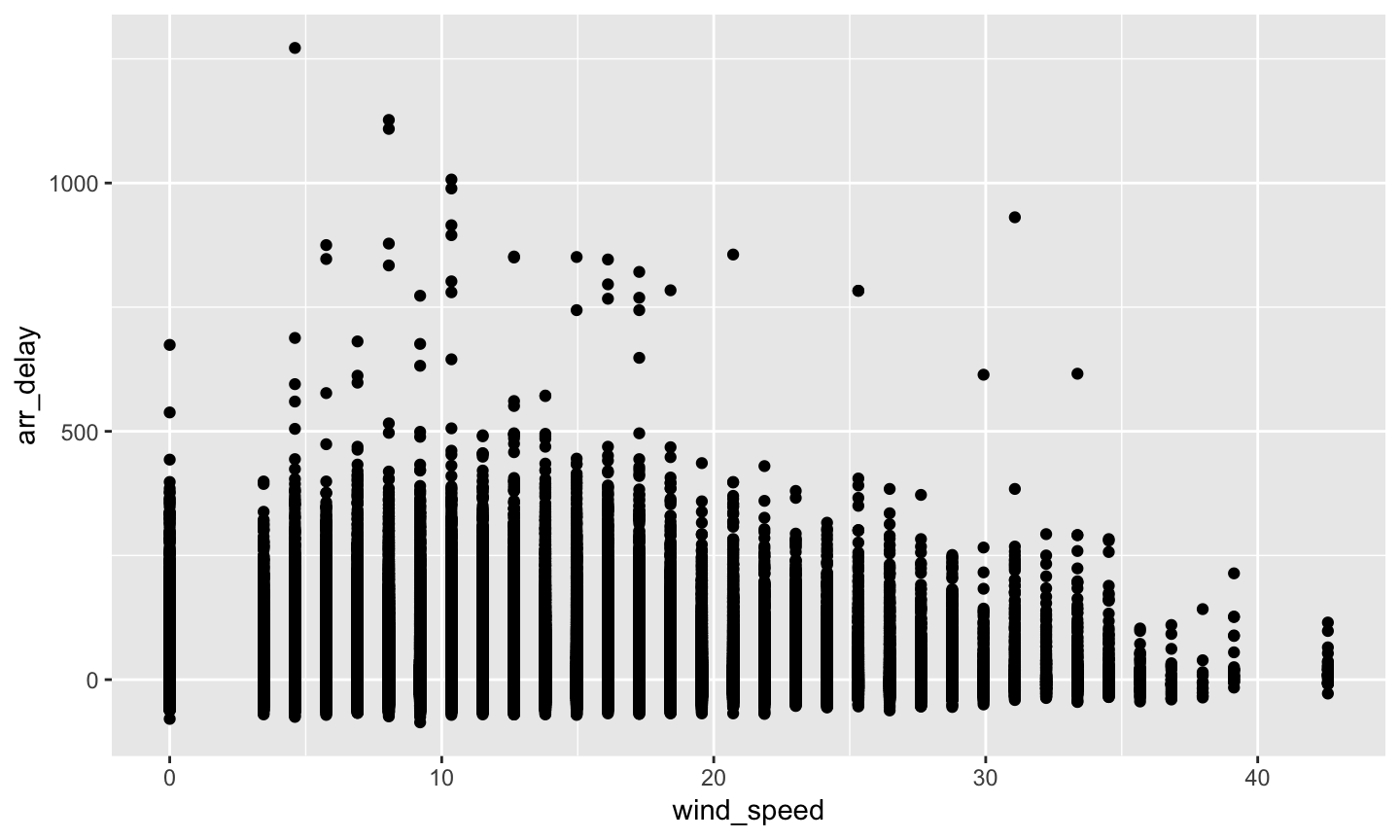
小練習

重新畫圖

left_join(flights, weather) %>%
  select(wind_speed, arr_delay) %>%
  filter(!is.na(wind_speed), !is.na(arr_delay)) %>%
  filter(wind_speed < 1000) %>%
  ggplot(aes(x = wind_speed, y = arr_delay)) +
  geom_point()

小練習

重新畫圖

## Joining, by = c("year", "month", "day", "origin", "hour", "time_hour")

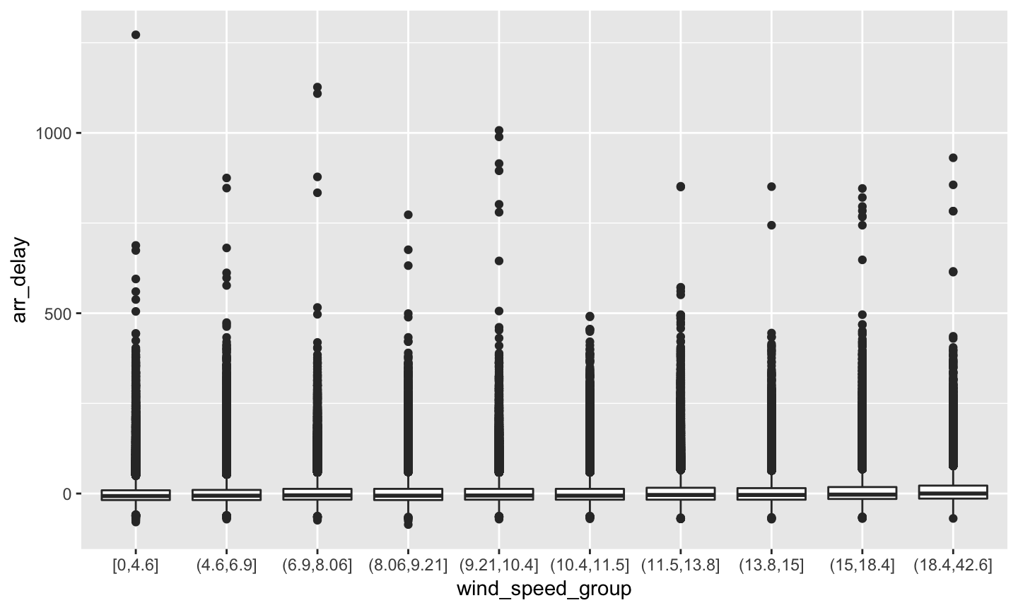
小練習

分組後取平均

.df <- left_join(flights, weather) %>%
  select(wind_speed, arr_delay) %>%
  filter(!is.na(wind_speed), !is.na(arr_delay)) %>%
  filter(wind_speed < 1000)
.cut <- quantile(.df$wind_speed, seq(0, 1, 0.1))
.df$wind_speed_group <- cut(.df$wind_speed, breaks = .cut, include.lowest = TRUE)
ggplot(.df, aes(x = wind_speed_group, y = arr_delay)) +
  geom_boxplot()

小練習

分組後取平均

## Joining, by = c("year", "month", "day", "origin", "hour", "time_hour")

小練習

分組後的分佈圖

.df <- left_join(flights, weather) %>%
  select(wind_speed, arr_delay) %>%
  filter(!is.na(wind_speed), !is.na(arr_delay)) %>%
  filter(wind_speed < 1000)
.cut <- quantile(.df$wind_speed, seq(0, 1, 0.1))
.df$wind_speed_group <- cut(.df$wind_speed, breaks = .cut, include.lowest = TRUE)
ggplot(.df, aes(x = wind_speed_group, y = arr_delay)) +
  geom_boxplot()

小練習

分組後的分佈圖

## Joining, by = c("year", "month", "day", "origin", "hour", "time_hour")

小練習

直接取平均

.df <- left_join(flights, weather) %>%
  select(wind_speed, arr_delay) %>%
  filter(!is.na(wind_speed), !is.na(arr_delay)) %>%
  filter(wind_speed < 1000)
.cut <- quantile(.df$wind_speed, seq(0, 1, 0.1))
.df$wind_speed_group <- cut(.df$wind_speed, breaks = .cut, include.lowest = TRUE)
group_by(.df, wind_speed_group) %>%
  summarise(mean(arr_delay))

小練習

直接取平均

## Joining, by = c("year", "month", "day", "origin", "hour", "time_hour")

## # A tibble: 10 x 2
##    wind_speed_group `mean(arr_delay)`
##    <fct>                        <dbl>
##  1 [0,4.6]                       3.52
##  2 (4.6,6.9]                     3.79
##  3 (6.9,8.06]                    6.23
##  4 (8.06,9.21]                   5.70
##  5 (9.21,10.4]                   6.17
##  6 (10.4,11.5]                   5.81
##  7 (11.5,13.8]                   8.35
##  8 (13.8,15]                     8.22
##  9 (15,18.4]                    10.4 
## 10 (18.4,42.6]                  13.1

小練習

去除邊界10%的資料後取平均

.df <- left_join(flights, weather) %>%
  select(wind_speed, arr_delay) %>%
  filter(!is.na(wind_speed), !is.na(arr_delay)) %>%
  filter(wind_speed < 1000)
.cut <- quantile(.df$wind_speed, seq(0, 1, 0.1))
.df$wind_speed_group <- cut(.df$wind_speed, breaks = .cut, include.lowest = TRUE)
group_by(.df, wind_speed_group) %>%
  summarise(mean(arr_delay, trim = 0.05))

小練習

去除邊界10%的資料後取平均

## Joining, by = c("year", "month", "day", "origin", "hour", "time_hour")

## # A tibble: 10 x 2
##    wind_speed_group `mean(arr_delay, trim = 0.05)`
##    <fct>                                     <dbl>
##  1 [0,4.6]                                  -1.90 
##  2 (4.6,6.9]                                -1.28 
##  3 (6.9,8.06]                                0.728
##  4 (8.06,9.21]                               0.204
##  5 (9.21,10.4]                               0.514
##  6 (10.4,11.5]                               0.414
##  7 (11.5,13.8]                               2.55 
##  8 (13.8,15]                                 2.40 
##  9 (15,18.4]                                 4.34 
## 10 (18.4,42.6]                               7.37

這些設定沒有標準答案

一定要用quantile切割資料嘛？
- 一定要十組嘛？
高手會調這些參數調到支持他們的論點
新手會亂改數據造假

其他的`join`函數

?left_join

`left_join`

兩個範例資料

band_members

## # A tibble: 3 x 2
##   name  band   
##   <chr> <chr>  
## 1 Mick  Stones 
## 2 John  Beatles
## 3 Paul  Beatles

band_instruments

## # A tibble: 3 x 2
##   name  plays 
##   <chr> <chr> 
## 1 John  guitar
## 2 Paul  bass  
## 3 Keith guitar

`left_join`

left_join(band_members, band_instruments)

## Joining, by = "name"

## # A tibble: 3 x 3
##   name  band    plays 
##   <chr> <chr>   <chr> 
## 1 Mick  Stones  <NA>  
## 2 John  Beatles guitar
## 3 Paul  Beatles bass

`right_join`

right_join(band_members, band_instruments)

## Joining, by = "name"

## # A tibble: 3 x 3
##   name  band    plays 
##   <chr> <chr>   <chr> 
## 1 John  Beatles guitar
## 2 Paul  Beatles bass  
## 3 Keith <NA>    guitar

`inner_join`

inner_join(band_members, band_instruments)

## Joining, by = "name"

## # A tibble: 2 x 3
##   name  band    plays 
##   <chr> <chr>   <chr> 
## 1 John  Beatles guitar
## 2 Paul  Beatles bass

`full_join`

full_join(band_members, band_instruments)

## Joining, by = "name"

## # A tibble: 4 x 3
##   name  band    plays 
##   <chr> <chr>   <chr> 
## 1 Mick  Stones  <NA>  
## 2 John  Beatles guitar
## 3 Paul  Beatles bass  
## 4 Keith <NA>    guitar

`anti_join`

anti_join(band_members, band_instruments)

## Joining, by = "name"

## # A tibble: 1 x 2
##   name  band  
##   <chr> <chr> 
## 1 Mick  Stones

`semi_join`

semi_join(band_members, band_instruments)

## Joining, by = "name"

## # A tibble: 2 x 2
##   name  band   
##   <chr> <chr>  
## 1 John  Beatles
## 2 Paul  Beatles

當y的Key有重複時，inner_join會重複， semi_join不會

時間資料的處理

Open Data上最常見於整合用的Key

時間
空間

時間整合的挑戰

時間格式不同
時間頻率不同

時間的格式: `format`

Sys.time()

## [1] "2019-05-11 02:55:35 CST"

format(Sys.time())

## [1] "2019-05-11 02:55:35"

format(Sys.time(), "%Y-%m-%d %H:%M:%S")

## [1] "2019-05-11 02:55:35"

format(Sys.time(), "%Y%m%d%H%M%S")

## [1] "20190511025535"

時間的格式: `format`

?format.POSIXct

Details 中有如%a的格式說明
我常用的
- "%Y-%m-%d %H:%M:%S" 年-月-日小時-分鐘-秒數，並且固定數字的位數

時間的格式: 實務上請愛用 ISO 8601

"%Y-%m-%dT%H:%M:%SZ"

R中的時間相關物件：`POSIXct`與`POSIXlt`

Sys.time()

## [1] "2019-05-11 02:55:35 CST"

class(Sys.time())

## [1] "POSIXct" "POSIXt"

strptime("2018-01-01 08:00:00", "%Y-%m-%d %H:%M:%S")

## [1] "2018-01-01 08:00:00 CST"

strptime("2018-01-01 08:00:00", "%Y-%m-%d %H:%M:%S") %>% class()

## [1] "POSIXlt" "POSIXt"

strptime("2018-01-01 08:00:00", "%Y-%m-%d %H:%M:%S") %>%
  as.POSIXct()

## [1] "2018-01-01 08:00:00 CST"

`POSIXct`的本質

從某個時間點（預設是格林威治時間1970-01-01 00:00:00）開始到指定時間為止的秒數
numeric vector

unclass(Sys.time())

## [1] 1557514536

`POSIXlt`的本質

分別紀錄年月日… 等資訊
list

unclass(strptime("2018-01-01 08:00:00", "%Y-%m-%d %H:%M:%S"))

## $sec
## [1] 0
## 
## $min
## [1] 0
## 
## $hour
## [1] 8
## 
## $mday
## [1] 1
## 
## $mon
## [1] 0
## 
## $year
## [1] 118
## 
## $wday
## [1] 1
## 
## $yday
## [1] 0
## 
## $isdst
## [1] 0
## 
## $zone
## [1] "CST"
## 
## $gmtoff
## [1] NA

個人比較常用`POSIXct`

dplyr有支援<dttm>
可以使用as.POSIXct
從某個時間點（預設是格林威治時間1970-01-01 00:00:00）開始到指定時間為止的秒數
與文字作轉換時要考慮時差、時區

.t <- 0
class(.t) <- class(Sys.time())
.t # Our timezone is +8

## [1] "1970-01-01 08:00:00 CST"

時區

我們要怎麼處理以下的時間：
- 台北時間 2018-01-01 08:00:00
- 格林威治時間 2018-01-01 00:00:00

as.POSIXct("2018-01-01 08:00:00", tz = "Asia/Taipei") %>% unclass()

## [1] 1514764800
## attr(,"tzone")
## [1] "Asia/Taipei"

as.POSIXct("2018-01-01 00:00:00", tz = "GMT") %>% unclass()

## [1] 1514764800
## attr(,"tzone")
## [1] "GMT"

時區

POSIXct: 與格林威治時間1970-01-01 00:00:00 (台北時間 1970-01-01 08:00:00)差距的秒數
- 台北時間 2018-01-01 08:00:00 與台北時間 1970-01-01 08:00:00 差 1514764800 秒
- 格林威治時間 2018-01-01 00:00:00 與格林威治時間 1970-01-01 00:00:00 也差 1514764800 秒

t <- 1514764800
class(t) <- class(Sys.time())
format(t)

## [1] "2018-01-01 08:00:00"

format.POSIXct(t, tz = "GMT") # S3

## [1] "2018-01-01"

時區

沒有指定時區時，R 預設會用Sys.timezone()

Sys.timezone()

## [1] "Asia/Taipei"

as.POSIXct("1970-01-01 00:00:00") %>% as.numeric()

## [1] -28800

時區

指定時區

as.POSIXct("1970-01-01 00:00:00", tz = "GMT") %>% as.numeric()

## [1] 0

總結

時間格式是以numeric vector的形式儲存
- 使用class修飾
不同時區的時間，只要對應到相同的時間點，則儲存的數值應該相同
- 台北時間 2018-01-01 08:00:00 與格林威治時間 2018-01-01 00:00:00 相同
時區會影響到時間的數值與時間的文字之間的轉換
- as.POSIXct: 文字 —> 數值
- format.POSIXct: 數值 —> 文字

轉換頻率

# 分
format(Sys.time(), "%M") %>% as.integer()

## [1] 55

# 時
format(Sys.time(), "%H") %>% as.integer()

## [1] 2

# 日
format(Sys.time(), "%d") %>% as.integer()

## [1] 11

轉換頻率

# 月
format(Sys.time(), "%m") %>% as.integer()

## [1] 5

# 年
format(Sys.time(), "%Y") %>% as.integer()

## [1] 2019

# 季
(format(Sys.time(), "%m") %>% as.integer() - 1) %/% 3

## [1] 1

# try (1:12 - 1) %/% 3

當時間的尺度不一致

GDP是每年一次的資料 v.s. 房貸餘額是每月一次的資料
- 將房貸餘額加總成為GDP(但是房貸餘額能加總嘛？)
- 找一個時間點的房貸餘額代表該年度的房貸餘額（要找幾月？）

大綱

讀取CSV

CSV的格式

read.csv

read.table

read.csv與read.table的注意事項

讀取CSV的可能錯誤：編碼問題

讀取CSV的可能錯誤：欄位數量不一致

小挑戰

讀取CSV檔案的小撇步: colClasses 參數

讀取CSV檔案的小撇步: colClasses 參數

讀取CSV檔案的小撇步: colClasses 參數

讀取CSV檔案的小撇步: colClasses 參數

Database

Transaction

Transaction

Transaction

XML Tables

2018 縣市長大選台北即時估票

data.frame

data.frame 的 Create

data.frame 的 Create

data.frame 的 Read

data.frame 的 Read

data.frame 的 Read

data.frame 的 Read

data.frame 的 Read

data.frame 的 Read

data.frame 的 Read

data.frame 的 Update

data.frame 的 Delete

範例

範例

範例

範例

範例

範例

範例

範例

範例

dplyr

參考SQL 資料庫系統對結構化資料的操作做設計

dplyr 沒有完全相容於 data.frame

Single Table verbs

針對列作篩選：filter

針對列作篩選：filter

針對列作篩選：filter

針對列作篩選：filter

針對列作篩選：filter

針對列作篩選：slice

針對列作抽樣：sample_n、sample_frac

針對欄位作篩選：select

針對欄位作篩選：select

針對欄位作篩選：select

針對欄位作篩選：select

針對欄位作篩選：select

針對欄位作篩選：select

更改資料(向量化)

更改資料(向量化)

Aggregation: summarise

Aggregation: summarise

Aggregation: do

Aggregation的目的

Aggregation: group_by

Aggregation: group_by + summarise

filter –> group_by

filter –> group_by

Aggregation

Aggregation: group_by + summarise

Aggregation: group_by + summarise

Aggregation: group_by + do

Aggregation: group_by + summarise

Aggregation: group_by + do

小挑戰

參考答案

參考答案

從dplyr到SQL

從dplyr到SQL

從dplyr到SQL

從dplyr到SQL

`read.csv`

`read.table`

`read.csv`與`read.table`的注意事項

讀取`CSV`的可能錯誤：編碼問題

讀取`CSV`的可能錯誤：欄位數量不一致

針對列作抽樣：`sample_n`、`sample_frac`

Aggregation: `group_by`

Aggregation: `group_by` + `summarise`

`filter` –> `group_by`

`filter` –> `group_by`

Aggregation: `group_by` + `summarise`

Aggregation: `group_by` + `summarise`

Aggregation: `group_by` + `do`

Aggregation: `group_by` + `summarise`

Aggregation: `group_by` + `do`

從`dplyr`到SQL

從`dplyr`到SQL

從`dplyr`到SQL

從`dplyr`到SQL

從`dplyr`到SQL

對`iris`計算各個Species的平均

對`iris.tall`計算各個Species的平均

對`iris.tall`計算各個Species的平均

解決辦法：pipeline operator `%>%`

`%>%` 細解

`%>%` 與 `.`

Key: `carrier`

`dplyr::left_join`

`dplyr::left_join`

`dplyr::left_join`的參數

`dplyr::left_join`: `by`參數

`y`上不唯一的Key

`y`上不唯一的Key

直接`left_join`

`airports`

`airports`

`airports`

`airports`